Notes On The Graphics Pipeline
Computer Graphics is a pretty interesting field. For instance, you can make a state of the art offline renderer without ever touching graphics hardware. When it comes to real-time rendering though, there’s no way around it, you have to use a GPU. And if you want to get good performance you have to use it well, and that begins with understanding the graphics pipeline.
The graphics pipeline is the name given to the stages data goes through in a graphics system in order to produce a rendered image. Back in the early days of accelerated graphics these stages worked like black boxes with a few knobs and switches to control their behavior, but over time some stages became programmable through small programs called shaders which give developers more control over the rendering process. Modern GPUs have very generic “shader cores” which can efficiently execute work from different programmable stages, so what distinguishes these stages is mostly the data that is being processed. Its up to the pipeline then to make sure data goes in and out of each stage as efficiently as possible.
Since the end goal of the rendering process is to produce an image with a few million pixels from a 3D scene with maybe a few million triangles, and given that there’s a limit to how fast you can process each piece of data, it’s imperative that as much of it as possible is processed in parallel. This is the guiding principle of GPUs, which work by having several of the aforementioned shader cores operating in parallel on many different data points. We’re going to see that its up to the developer to utilize these cores efficiently, trying to keep as many of them occupied with work as possible.
The Pipeline
Below we have a simplified diagram for the pipeline stages with the optional tesselation and geometry shader stages omitted. We’re going to assume we have vertex and index data sitting in GPU memory and that the command processor has configured the pipeline and set it to work on drawing a frame, in order to follow how the data goes through each stage to produce the final image.
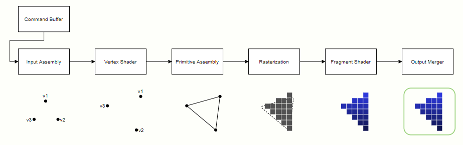
Input Assembly
After the draw command is issued, the first stage in the pipeline is the Input Assembly, whose job it is to read the indices in the index buffer and use them to assemble a block of data with the primitive’s vertices, which will be sent to the Vertex Shader. These vertices are cached to avoid shading a vertex shared by multiple primitives more than once. Usually all vertices of a primitive are placed in the same block, so the Primitive Assembly stage down the line doesn’t have to wait for multiple blocks of work from the Vertex Shader.
Vertex Shader
This is the first programmable stage in the pipeline. It receives a block of vertices and executes a shader program that is responsible for applying per-vertex operations, such as the transformation from object space to clip space.
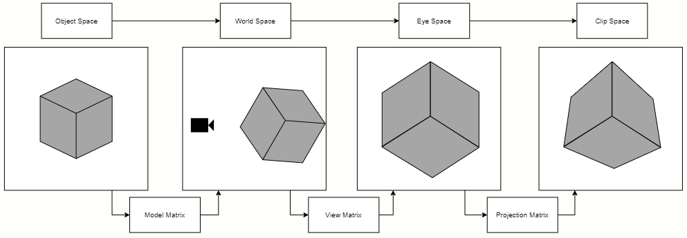
An object’s vertices exist in a space called object space, where vertex positions are defined in relation to the object’s origin. In order to transform them to clip space, matrix multiplications are used. First the vertices are multiplied by a model matrix to get their world coordinates. Then they’re multiplied by a view matrix, which transforms them so they’re viewed from a camera’s perspective. Finally a projection matrix applies either a perspective or orthogonal transformation, projecting the vertices onto a 2D plane. This projection brings them to the so called clip space, which, as the name suggests, is the space where primitives will be clipped against the view frustum (the observable space from the camera’s point of view) in the next stage of the pipeline.
Besides transformations, in the Vertex Shader stage additional attributes can be attached to each vertex. These attributes along with the vertex positions will be interpolated and provided to the Fragment Shader.
Primitive Assembly
This stage receives the transformed block of vertices from the Vertex Shader. As mentioned before, all vertices of a primitive are expected to be in a same block, so as soon as a block is received the primitive assembly can start doing its job of gathering all vertices belonging to a primitive, which is usually a triangle.
Primitives that intersect the bounds of the view frustum are then clipped so their coordinates are contained within the [-w, w] range, where w is the homogeneous coordinate of the vertex. Clipped primitives are then transformed into NDC space (normalized device coordinates), which basically means dividing the coordinates by w so they lie in the [-1, 1] range. Finally they’re transformed into screen space by mapping the [-1, 1] range to the screen size.
The final step of this stage applies triangle culling. The signed area of each triangle is calculated, so we can tell if the triangle is front-facing (positive area), back-facing (negative area) or degenerate (zero area). Degenerate triangles are always discarded, and front- and back-facing triangles are discarded according to the pipeline setup.
Rasterization
Rasterization is responsible for taking vector equations derived from a primitive’s vertices and deducing which pixels correspond to the primitive. Usually it’s implemented in a coarse and a fine stage. In the coarse stage, the screen is divided into large blocks which are tested to see if they intersect with the primitive (this is called a coverage test). Coarse blocks that intersect it are then forwarded to the fine stage, where they’re divided into smaller blocks, which are then tested for coverage at the pixel level. The smaller blocks are separated into quads (blocks of 2x2 pixels), and quads which have at least one intersecting pixel are sent to the next stage, where their attributes will be interpolated before being used.
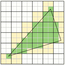
When multisample antialiasing is enabled, instead of testing a single pixel the corresponding number of subpixels are tested. Only the actual pixel will be shaded in the next stage, but the ratio of subpixels that are covered by the primitive will determine how the pixel color will be blended in the final image, in a step called MSAA resolve. For example if we use 4x MSAA, if the background is black and we draw a white pixel that has only 2 covered subpixels (out of 4), the resolved pixel color will be 50% black and 50% white, ie. gray.
One important thing to note here is that the fact that pixels are sent to the next stage in quads means that we may end up wasting resources. For example, if only a single pixel in a quad is covered by a primitive, we’ll still have to process a full quad, but 75% of the work will be discarded. This is called quad overdraw, and happens mostly with very small or very thin triangles, which might end up impacting performance.
Fragment Shader
This is another programmable stage in the pipeline. It receives a block of pixels with their interpolated position and attributes, and executes a shader program that is responsible for applying per-pixel operations (such as lighting), outputting a shaded pixel.
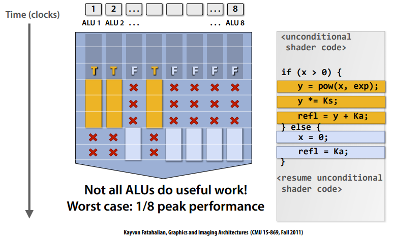
Like the Vertex Shader, this stage receives a block of data which is then divided into smaller batches that “fit” in a shader core. This is done because in hardware each core can run instructions on many points of data at the same time. If, say, the core can run 16 threads per cycle, then 4 quads (each with 4 points of data, which in this case will be pixels) can be processed at once. For all of the pixels in these quads the code of the fragment shader will execute with the exact same instructions being run at each clock cycle (in lockstep). This can become problematic when the pixel shader has branches, since if a single thread enters a branch, the others will have to stall until they can continue execution, so developers have to manage this efficiently.
When quad overdraw happens, you can have 75% of threads shading pixels that will be discarded, which is a massive waste of resources. Why not just process each pixel individually then? The reason is derivatives, which are used by texture samplers to select mip levels and perform filtering. If every pixel is placed in a quad along with its neighbors, the derivatives can be easily calculated.
After the Fragment Shader is executed, the shaded quads are sent to the final stage of the pipeline.
Output Merger
The Output Merger stage is where the final pixel color is generated according to pipeline state, the quads received from the Fragment Shader, the contents of bound render targets as well as depth/stencil buffers. First depth and stencil tests are performed to see if the incoming pixels should be discarded. If they pass the tests, the color of each pixel is then blended with the contents of the render target, performing MSAA resolve if necessary. The final pixel is then written back to the render target and compression is applied.
And that’s it. That’s the end of the journey for the data, which went from vertices and indices to shaded pixels that can now be presented to the screen. Somethings we didn’t cover are Tesselation and Geometry Shaders, which sit between the Vertex Shader and the Primitive Assembly stage, and the Compute Pipeline, which is way simpler having only a single programmable stage. If you’re interested in learning more, check out the resources below.